Simulating Multiple-Orbital Systems
In this section, we will see how to generate the multiorbital Hamiltonian for a moiré system and compute its band structure. This is essential for understanding the interplay between orbital degrees of freedom and moiré-induced electronic structure. This notebook shows a compact k=2 setup where each hopping can be a 2x2 block.
!!! Here, k denotes the number of orbitals per site and should not be confused with the K-points in momentum space.
1. Setup
We define the lattice once with k=2 and reuse it in all later cells.
import numpy as np
import matplotlib.pyplot as plt

from moirepy import BilayerMoireLattice, TriangularLayer

lattice = BilayerMoireLattice(
    latticetype=TriangularLayer,
    ll1=2,
    ll2=3,
    ul1=3,
    ul2=2,
    n1=1,
    n2=1,
    k=2,
    pbc=True,
)

lattice.generate_connections(inter_layer_radius=1.0)


# Output:
# twist angle = 0.2299 rad (13.1736 deg)
# 19 cells in upper lattice
# 19 cells in lower lattice
2. Build a Block Hamiltonian
Here we mix scalar and matrix-valued inputs:
- In general the t's should be functions that take in certain parameters (as shown in custom_hoppings file) and returns k x k blocks, where k is the number of orbitals per site. But here are some relaxations to the rule.
- If the hopping is supposed to remain constant across the lattice, you can directly input the k x k block without wrapping it in a function.
- If the hopping between any two orbitals is the same, you can directly input a scalar. The code will automatically broadcast it to a full k x k block.
- If the hopping between any two orbitals is the same, but it is different across the lattice, you can input a function that returns a scalar. The code will automatically broadcast it to a full k x k block.
real_ham = lattice.generate_hamiltonian(
    tll=0.3,
    tuu=0.0,
    tul=(
        (0.8, 0.5),
        (0.5, 0.8),
    ),
    tlu=1.0,
    tuself=0.2,
    tlself=(
        (0.4, 0.1),
        (0.1, 0.4),
    ),
    data_type=np.float64,  # default is np.complex128
).toarray()  # convert to dense array for visualization purposes

print("Hamiltonian shape:", real_ham.shape)

# Output:
# Hamiltonian shape: (76, 76)
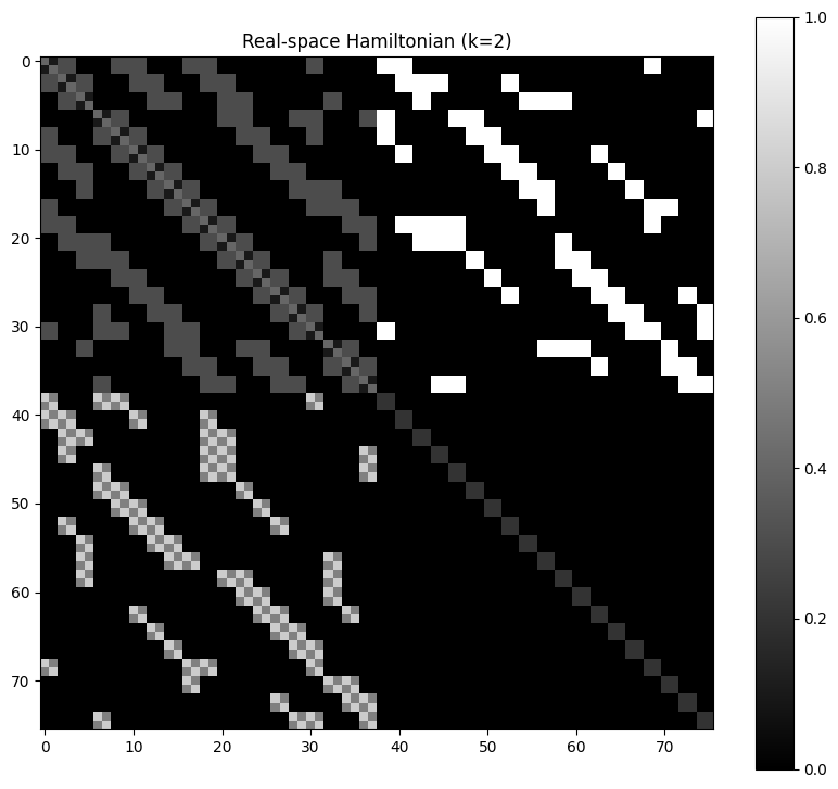
3. Visualize Matrix Structure
plt.figure(figsize=(10, 9))
plt.imshow(real_ham, cmap='gray')
plt.title('Real-space Hamiltonian (k=2)')
plt.colorbar()

# Output:
# <matplotlib.colorbar.Colorbar at 0x7260fbf016a0>
4. Inspect a Small Block
print(real_ham[:16, :16])

# Output:
# [[0.4 0.1 0.3 0.3 0.  0.  0.  0.  0.3 0.3 0.3 0.3 0.  0.  0.  0. ]
#  [0.1 0.4 0.3 0.3 0.  0.  0.  0.  0.3 0.3 0.3 0.3 0.  0.  0.  0. ]
#  [0.3 0.3 0.4 0.1 0.3 0.3 0.  0.  0.  0.  0.3 0.3 0.3 0.3 0.  0. ]
#  [0.3 0.3 0.1 0.4 0.3 0.3 0.  0.  0.  0.  0.3 0.3 0.3 0.3 0.  0. ]
#  [0.  0.  0.3 0.3 0.4 0.1 0.  0.  0.  0.  0.  0.  0.3 0.3 0.3 0.3]
#  [0.  0.  0.3 0.3 0.1 0.4 0.  0.  0.  0.  0.  0.  0.3 0.3 0.3 0.3]
#  [0.  0.  0.  0.  0.  0.  0.4 0.1 0.3 0.3 0.  0.  0.  0.  0.  0. ]
#  [0.  0.  0.  0.  0.  0.  0.1 0.4 0.3 0.3 0.  0.  0.  0.  0.  0. ]
#  [0.3 0.3 0.  0.  0.  0.  0.3 0.3 0.4 0.1 0.3 0.3 0.  0.  0.  0. ]
#  [0.3 0.3 0.  0.  0.  0.  0.3 0.3 0.1 0.4 0.3 0.3 0.  0.  0.  0. ]
#  [0.3 0.3 0.3 0.3 0.  0.  0.  0.  0.3 0.3 0.4 0.1 0.3 0.3 0.  0. ]
#  [0.3 0.3 0.3 0.3 0.  0.  0.  0.  0.3 0.3 0.1 0.4 0.3 0.3 0.  0. ]
#  [0.  0.  0.3 0.3 0.3 0.3 0.  0.  0.  0.  0.3 0.3 0.4 0.1 0.3 0.3]
#  [0.  0.  0.3 0.3 0.3 0.3 0.  0.  0.  0.  0.3 0.3 0.1 0.4 0.3 0.3]
#  [0.  0.  0.  0.  0.3 0.3 0.  0.  0.  0.  0.  0.  0.3 0.3 0.4 0.1]
#  [0.  0.  0.  0.  0.3 0.3 0.  0.  0.  0.  0.  0.  0.3 0.3 0.1 0.4]]
Summary
- Setting
k=2promotes each site to a2x2orbital block. - You can combine scalar terms with explicit
(k, k)matrices. - The generated Hamiltonian remains a standard sparse matrix, ready for downstream analysis.