Simulating Non-Hermitian Systems

This notebook presents a minimal non-Hermitian bilayer model in MoirePy. Non-Hermiticity is introduced through an angle-dependent in-plane hopping amplitude. For simplicity, the inter-layer hopping (t_lu = t_ul) is taken to be symmetric in this example. However, there is no fundamental restriction within the framework, and fully general non-Hermitian systems can be constructed in the same way.

1. Setup

We build one lattice instance with open boundary conditions and reuse it throughout.

import numpy as np
import matplotlib.pyplot as plt

from moirepy import BilayerMoireLattice, SquareLayer

params = {
    "latticetype": SquareLayer,
    "ll1": 9,
    "ll2": 10,
    "ul1": 10,
    "ul2": 9,
    "n1": 1,
    "n2": 1,
}

lattice = BilayerMoireLattice(**params, pbc=False)
lattice.generate_connections(inter_layer_radius=1.0)

# Output:
# twist angle = 0.1052 rad (6.0256 deg)
# 181 cells in upper lattice
# 181 cells in lower lattice

2. Direction-Dependent Intra-Layer Hopping

The callable below follows the pair-hopping signature and returns one value per bond.

def anisotropic_hopping(pos_i, pos_j, R, type_i, type_j, lattice, t0=1.0, gamma=0.3):
    # Vectorized bond directions in the lattice frame.
    d = (pos_j + R) - pos_i
    theta = np.arctan2(d[:, 1], d[:, 0])
    return t0 + gamma * np.cos(theta)

3. Build a Non-Hermitian Hamiltonian

We set tlu and tul to different constants to make the Hamiltonian non-Hermitian.

ham = lattice.generate_hamiltonian(
    tll=anisotropic_hopping,
    tuu=anisotropic_hopping,
    tlu=1.0,
    tul=1.0,
    tlself=0.0,
    tuself=0.0,
).toarray()

print("Is the Hamiltonian Hermitian?", np.allclose(ham, ham.conj().T))

# Output:
# Is the Hamiltonian Hermitian? False

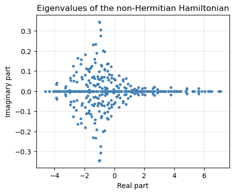
4. Complex Spectrum

e, v = np.linalg.eig(ham)

plt.figure(figsize=(5, 4))
plt.plot(e.real, e.imag, 'o', color='steelblue', markersize=3)
plt.xlabel('Real part')
plt.ylabel('Imaginary part')
plt.title('Eigenvalues of the non-Hermitian Hamiltonian')
plt.grid(alpha=0.3)

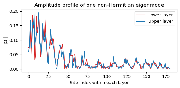
5. One Eigenmode (Skin-Effect Style Localization)

mode = np.argmax(np.abs(e.imag))
amp = np.abs(v[:, mode])

n_lower = lattice.lower_lattice.points.shape[0]

plt.figure(figsize=(6, 3))
plt.plot(amp[:n_lower], label='Lower layer', color='tab:red')
plt.plot(amp[n_lower:], label='Upper layer', color='tab:blue')
plt.xlabel('Site index within each layer')
plt.ylabel('|psi|')
plt.title('Amplitude profile of one non-Hermitian eigenmode')
plt.legend()
plt.tight_layout()

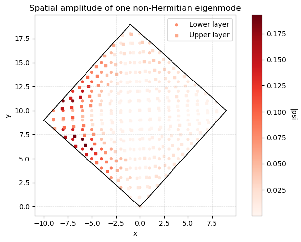
6. Spatial Eigenmode Amplitude on the Lattice

This reproduces the geometric view from section 7 in custom_hoppings.ipynb: we color each lattice site by the eigenmode amplitude.

# Spatial plot of one eigenmode on the moire geometry
mode = np.argmax(np.abs(e.imag))

n_lower = lattice.lower_lattice.points.shape[0]
amp_lower = np.abs(v[:n_lower, mode])
amp_upper = np.abs(v[n_lower:, mode])

plt.figure(figsize=(7, 5))

nx = lattice.n1
ny = lattice.n2
mlv1 = lattice.mlv1
mlv2 = lattice.mlv2

# Draw simulation supercell boundary
plt.plot([0, nx * mlv1[0]], [0, nx * mlv1[1]], 'k', linewidth=1)
plt.plot([0, ny * mlv2[0]], [0, ny * mlv2[1]], 'k', linewidth=1)
plt.plot(
    [nx * mlv1[0], nx * mlv1[0] + ny * mlv2[0]],
    [nx * mlv1[1], nx * mlv1[1] + ny * mlv2[1]],
    'k',
    linewidth=1,
)
plt.plot(
    [ny * mlv2[0], nx * mlv1[0] + ny * mlv2[0]],
    [ny * mlv2[1], nx * mlv1[1] + ny * mlv2[1]],
    'k',
    linewidth=1,
)

# Draw one moire unit cell
plt.plot([0, mlv1[0]], [0, mlv1[1]], 'k--', linewidth=1)
plt.plot([0, mlv2[0]], [0, mlv2[1]], 'k--', linewidth=1)
plt.plot([mlv1[0], mlv1[0] + mlv2[0]], [mlv1[1], mlv1[1] + mlv2[1]], 'k--', linewidth=1)
plt.plot([mlv2[0], mlv1[0] + mlv2[0]], [mlv2[1], mlv1[1] + mlv2[1]], 'k--', linewidth=1)

# Plot lower and upper layer sites colored by |psi|
sc_lower = plt.scatter(
    lattice.lower_lattice.points[:, 0],
    lattice.lower_lattice.points[:, 1],
    c=amp_lower,
    cmap='Reds',
    s=12,
    label='Lower layer',
)

plt.scatter(
    lattice.upper_lattice.points[:, 0],
    lattice.upper_lattice.points[:, 1],
    c=amp_upper,
    cmap='Reds',
    s=12,
    marker='s',
    label='Upper layer',
)

plt.gca().set_aspect('equal', adjustable='box')
plt.xlabel('x')
plt.ylabel('y')
plt.title('Spatial amplitude of one non-Hermitian eigenmode')
plt.grid(True, linestyle='--', linewidth=0.5, alpha=0.4)
plt.legend(loc='best')

cbar = plt.colorbar(sc_lower)
cbar.set_label('|psi|', rotation=270, labelpad=15)

plt.tight_layout()
plt.show()

Summary

• Non-Hermiticity is easy to model in MoirePy through asymmetric hopping choices.
• The resulting spectrum can become complex.
• Eigenmode amplitudes can show strong boundary/localization effects.