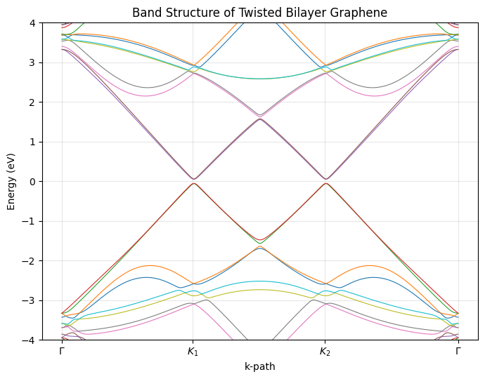
Electronic spectrum of twisted bilayer graphene (Nori et al.)
This notebook presents a clean implementation based on the paper:
A.O. Sboychakov, A.L. Rakhmanov, A.V. Rozhkov, Franco Nori
Electronic spectrum of twisted bilayer graphene (2015)
https://journals.aps.org/prb/abstract/10.1103/PhysRevB.92.075402
Code Author:
Sarbajit Mazumdar
Doctoral Researcher, Julius-Maximilians-Universitat Wurzburg
Email: sarbajit.mazumdar@uni-wuerzburg.de
Scope
- Build a commensurate twisted bilayer graphene lattice.
- Use a custom interlayer hopping with screening.
- Compute the band structure on a high-symmetry path.
- Estimate the band gap after centering the neutrality point.
Imports
import numpy as np
import matplotlib.pyplot as plt
from tqdm import tqdm

from moirepy import BilayerMoireLattice, Layer
Model parameters and graphene layer
Parameters used in this notebook:
The tuples ALPHA, BETA, and C_SCALE are the interlayer-hopping model parameters used in the current code.
A_GRAPHENE = 2.46
D_SPACING = 3.35
ALPHA = (6.715, 0.762, 0.179, 1.411)
BETA = (6.811, 0.01, 19.176)
C_SCALE = 1.44
T_INTRA = 2.57


class Graphene(Layer):
    def __init__(self, pbc=False, study_proximity: int = 1) -> None:
        lv1 = np.array([1.0, 0.0]) * A_GRAPHENE
        lv2 = np.array([0.5, np.sqrt(3.0) / 2.0]) * A_GRAPHENE

        basis_points = [
            (0.0, 0.0, "A"),
            (A_GRAPHENE, A_GRAPHENE / np.sqrt(3.0), "B"),
        ]

        neigh_deltas = np.array([
            [0.0, 1.0 / np.sqrt(3.0)],
            [-0.5, -1.0 / (2.0 * np.sqrt(3.0))],
            [0.5, -1.0 / (2.0 * np.sqrt(3.0))],
        ]) * A_GRAPHENE

        neighbours = {"A": neigh_deltas, "B": -neigh_deltas}
        super().__init__(lv1, lv2, basis_points, neighbours, pbc, study_proximity)
Build the commensurate twisted bilayer lattice
The active supercell choice below is (ll1,ll2,ul1,ul2)=(1,2,2,1).
ll1, ll2, ul1, ul2 = 1, 2, 2, 1

lattice = BilayerMoireLattice(
    Graphene,
    ll1,
    ll2,
    ul1,
    ul2,
    n1=1,
    n2=1,
    pbc=True,
    translate_upper=(-A_GRAPHENE, -A_GRAPHENE / np.sqrt(3.0)),
)

lattice.generate_connections(inter_layer_radius=A_GRAPHENE / (2.0 * np.sqrt(3.0)))

# Output:
# twist angle = 0.3803 rad (21.7868 deg)
# 14 cells in upper lattice
# 14 cells in lower lattice
Interlayer hopping model with screening
This section defines the screening function and interlayer coupling used by tul/tlu in Hamiltonian construction.
def screening_S(pos_i, pos_j, all_pos):
    rij = np.linalg.norm(pos_i - pos_j)
    ril = np.linalg.norm(all_pos - pos_i, axis=1)
    rjl = np.linalg.norm(all_pos - pos_j, axis=1)

    mask = (ril > 1e-6) & (rjl > 1e-6)
    x = ((ril[mask] + rjl[mask]) / rij).sum()
    xi = BETA[0] * np.exp(-BETA[1] * x**BETA[2])
    return np.tanh(xi)


def v_sigma(rij):
    r_scaled = C_SCALE * rij
    return ALPHA[0] * r_scaled ** (-ALPHA[1]) * np.exp(-ALPHA[2] * r_scaled ** ALPHA[3])


def t_perp_func(pos_u, pos_l, all_pos, d):
    rij = np.linalg.norm(pos_u - pos_l)
    inplane = np.linalg.norm(pos_u[:2] - pos_l[:2])
    cos_a = d / np.sqrt(d**2 + inplane**2)
    s_val = screening_S(pos_u, pos_l, all_pos)
    return (cos_a**2) * v_sigma(rij) * (1.0 - s_val)


def tul(pos_u, pos_l, R, type_u, type_l, lattice, d):
    lower_3d = np.column_stack([
        lattice.lower_lattice.bigger_points,
        np.zeros(len(lattice.lower_lattice.bigger_points)),
    ])
    upper_3d = np.column_stack([
        lattice.upper_lattice.bigger_points,
        np.full(len(lattice.upper_lattice.bigger_points), d),
    ])
    all_pos = np.vstack([lower_3d, upper_3d])

    vals = [
        t_perp_func(np.append(pu, d), np.append(pl, 0.0), all_pos, d)
        for pu, pl in zip(pos_u, pos_l + R)
    ]
    return np.array(vals)


def tlu(pos_l, pos_u, R, type_l, type_u, lattice, d):
    return np.conj(tul(pos_u, pos_l, R, type_u, type_l, lattice, d))
Reciprocal lattice and k-path
High-symmetry path used here:
def reciprocal_vectors(v1, v2):
    mat = np.column_stack([v1, v2])
    inv_t = 2.0 * np.pi * np.linalg.inv(mat).T
    return inv_t[:, 0], inv_t[:, 1]


g1, g2 = reciprocal_vectors(lattice.mlv1, lattice.mlv2)

gamma_point = np.zeros(2)
k1_point = (g1 + 2.0 * g2) / 3.0
k2_point = (2.0 * g1 + g2) / 3.0


def get_kpath(nseg):
    path_pts = [gamma_point, k1_point, k2_point, gamma_point]
    labels = [r"$\Gamma$", r"$K_1$", r"$K_2$", r"$\Gamma$"]

    k_list = []
    x_coords = []
    ticks = [0.0]
    tick_labels = [labels[0]]
    current_x = 0.0

    for i in range(len(path_pts) - 1):
        is_last = i == len(path_pts) - 2
        n_pts = nseg + 1 if is_last else nseg
        tvals = np.linspace(0.0, 1.0, n_pts, endpoint=is_last)

        segment = (1.0 - tvals)[:, None] * path_pts[i] + tvals[:, None] * path_pts[i + 1]
        k_list.extend(segment)
        x_coords.append(current_x + tvals)

        current_x = x_coords[-1][-1] + (0.0 if is_last else 1.0 / nseg)
        ticks.append(x_coords[-1][-1] if is_last else current_x - 1.0 / nseg)
        tick_labels.append(labels[i + 1])

    return np.array(k_list), np.concatenate(x_coords), ticks, tick_labels


k_points, x_ax, ticks, labels = get_kpath(100)
Build and diagonalize the Hamiltonian along the k-path
ham_real_space = lattice.generate_hamiltonian(
    tll=-T_INTRA,
    tuu=-T_INTRA,
    tul=tul,
    tlu=tlu,
    extra_inputs={"d": D_SPACING},
).toarray()

all_energies = []
for kvec in tqdm(k_points, desc="Diagonalizing H(k)"):
    phase = lattice.get_phase(kvec).toarray()
    ham_k = ham_real_space * phase
    eigvals = np.linalg.eigvalsh(ham_k)
    all_energies.append(eigvals)

all_energies = np.array(all_energies)

# Output:
# Diagonalizing H(k): 100%|██████████| 301/301 [00:00<00:00, 3417.59it/s]
Extract neutrality shift and estimate the gap
The two middle bands are used to estimate the valence-band maximum, conduction-band minimum, and gap.
mid_idx = all_energies.shape[1] // 2
lower_band = all_energies[:, mid_idx - 1]
upper_band = all_energies[:, mid_idx]

v_top = np.max(lower_band)
c_bottom = np.min(upper_band)
mu_shift = (v_top + c_bottom) / 2.0

gap = c_bottom - v_top
all_energies_shifted = all_energies - mu_shift

print(f"Chemical Potential Shift (mu): {mu_shift * 1e3:.2f} meV")
print(f"Calculated Band Gap: {gap * 1e3:.2f} meV")

# Output:
# Chemical Potential Shift (mu): 0.13 meV
# Calculated Band Gap: 108.73 meV
Plot the band structure
plt.figure(figsize=(7.0, 5.5))
plt.plot(x_ax, all_energies_shifted, lw=0.8)
plt.xticks(ticks, labels)
plt.xlabel("k-path")
plt.ylabel("Energy (eV)")
plt.ylim(-4.0, 4.0)
plt.title("Band Structure of Twisted Bilayer Graphene")
plt.grid(alpha=0.3)
plt.tight_layout()
plt.show()